Syzygy Analytics

Introduction

In the first part we looked at how goal scoring is affected by game state and found out that leading teams/trailing teams perform worse/better than would be expected respectively.  In this part we are going to look beyond goals and consider shots and xG. 

To start it will be illuminating to discover what effect losing/winning has on a team’s performance when we measure that performance using shots or xG.  I used xG data for 5 leagues from understat.com and shots using Opta data from whoscored.com.

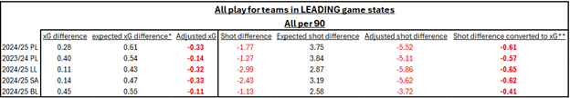
Table 1

*The expected difference is the performance we would expect based on the ability of the teams.  It’s always going to be positive on a large sample like a season because leading teams are always better teams on average.

**About 1 in 9 shots result in a goal.  To compare shot difference to xG difference it is divided by 9 for this final column.

We can see that shots are more affected by game state than xG – leading teams create more xG but shoot less than their opponents.  Adjusting the shot difference metric for game state will be a larger adjustment than the one for xG. 

Goals vs. xG

In the first article on game state, I focused on how goal difference is influenced by different game states.  It’s interesting to compare the xG figures from above to goal difference from table 2 in the first part of this series.  Pulling the data for the same 5 leagues from that table  

Table 2

The last 2 columns show a close agreement between the underperformance in goals and xG for each league.  This is a good thing for the understat xG model – game state does not influence goal conversion in a way that xG does not capture.

Adjusting a team’s performance for game state

As shown above, goals and the xG metric that understat.com uses are affected equally by game state so the following could be considered as an adjustment for either goal difference or xG difference. 

The purpose of a potential game state adjustment is to improve a metric so that it will become more predictive.  If a team is going to underperform whenever they lead, it follows that we don’t need to adjust for underperformance while leading in the past.

The relevant point is whether a team has led/trailed in different proportions than would be expected going forward.  If the team has trailed for a surprising number of minutes, they will have benefited from the trailing game state more than they will benefit from the trailing state when their trailing/leading minutes return to a more expected value.

In order to go about making this adjustment, firstly it is necessary to create a relationship between team performance and the expected leading/trailing minutes of said team.

Correlating some league data can give a relationship between performance and time trailing/leading.  The correlation used is xG difference for a team (i.e. performance) and fraction of time leading or trailing.  This gives an approximate relationship of:

1. Time expected to lead = 0.15 * xG diff. per 90 + 0.25
2. Time expected to trail = -0.15 * xG diff. per 90 + 0.25

Considering a league average team with a zero GD/xG, this shows on average they will spend 25% of the time trailing, 50% drawing and 25% leading. 

A team with a performance level of +0.5 xG diff per 90 is expected to spend 17.5% of the time trailing and 32.5% of the time leading. 

It’s useful to do 1) subtract 2).  This gives

• proportion of time leading – trailing = 0.3 * xG diff. per 90.

Using this formula for last year’s Premier League season gives the following table:

Premier League 2024/25 season adjustments

Table 3

• The first (numerical) column is the xG performance of each team. 
• This figure is used in formula 3. to create the second column. 
• The third column is the actual proportion of time each team spent winning and losing last season. 
• The fourth column uses the (global) value of -0.2 xG per game for winning teams to calculate the effect of game state using predicted time spent winning and losing.  E.g. Liverpool’s rating is so strong they are expected to spend 40.2% more time winning than they are losing.  This would damage their xG difference by 0.08 a game.  Southampton are expected to spend 47% more time losing which would benefit their xg difference by 0.09 a game.   
• The fifth column does the same calculation using each team’s actual time spent winning/losing. 
• The final column is our game state adjustment for xG (expected game state influence – actual game state influence).  Nottingham Forest for example spent a surprising number of minutes leading when considering their league average xG difference.  Their xG difference suffered because of this and as they are not expected to experience so many leading minutes going forward this results in a positive adjustment.  Bournemouth spent a surprisingly large number of minutes not winning and so their xG benefits because of this.

There are quite a lot of assumptions being made here:

• The blanket approximation that all teams underperform by 0.2 xG per 90 and overperformed by 0.2 xG per 90 while trailing may not hold.  There could be several reasons for this such as individual teams employing different styles in different game states or added nuance that I am yet to consider such as better teams not experiencing weaker performance while they lead.
• The ratings used for each team are accurate (for example I don’t think Bournemouth were/are as good as their xG difference which affects the game state adjustment.)

Shot difference adjustment

Table 4

• The game state adjustment for shots follows a similar process to xG.  Shot difference can be converted to an xG equivalent by diving the shot numbers by 9 (so formula 3 from above can be used).
• The game state effect for shots is around -5.1 per 90 for leading teams (which is a larger effect than -0.2xG per 90)
• I could do an iteration and use a GS adjusted shot difference per 90 rating for estimating expecting winning/losing times, but the result will not be significantly different.

Summary

Summarising the adjustments calculated for xG and shots:

The adjustments for shots are larger than the adjustments for xG.  Brentford are significantly underrated by just shot counts, but the game state adjustment helps to move that rating in the correct direction.   

These adjustments are fairly broad and make assumptions such as

1. Leading/trailing game state effects don’t change depending on the team in question
2. Leading/trailing game state effects don’t change depending on the minute of the game
3. Leading/trailing game state effects don’t change depending on the relative ability of the teams

Some of these may be reasonable assumptions but some may not. 

In the third part of my series of game state articles it will be interesting to look at how passing metrics are affected by game state.  These passing metrics could add an extra layer of depth to game state adjustments.

Thanks for reading and please get in touch about anything on x.com/samh112358

Also subscribe if you wish for notifications when I post new material!